How Do You Build a Production Computer Vision System?
Building production computer vision means pairing the right model with a data, deployment, and drift-monitoring pipeline.

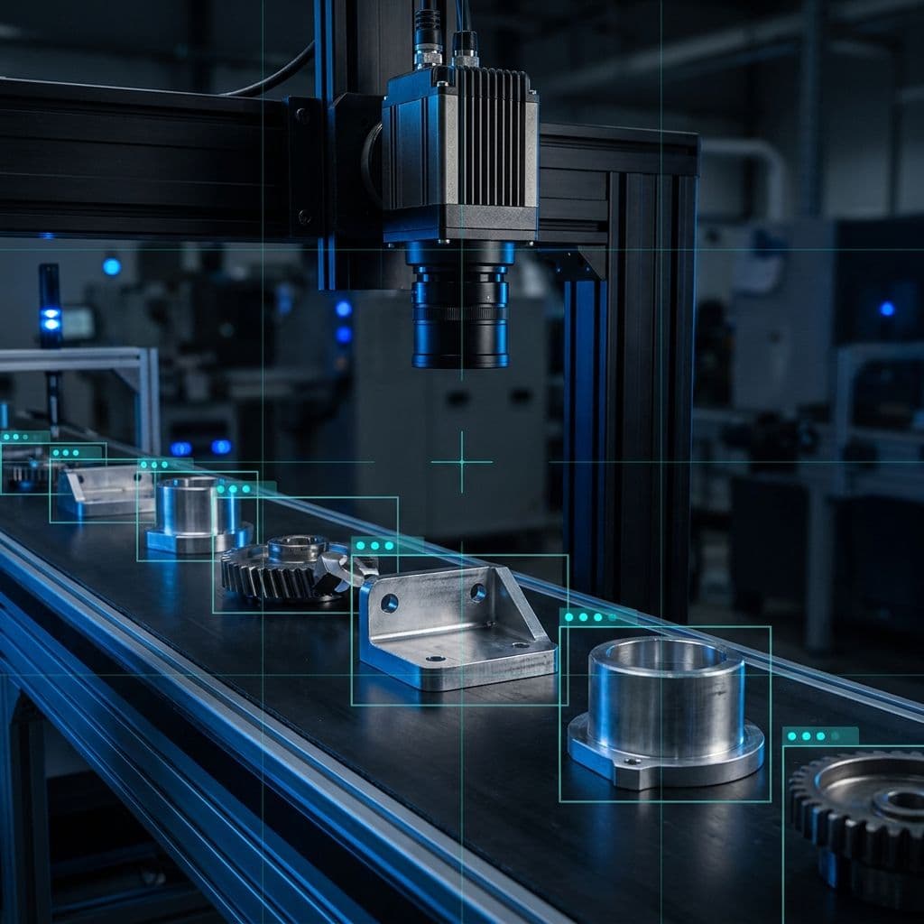
A production computer vision system is not a model — it is a pipeline: image capture, labeled data, a trained detector, an optimized runtime, and continuous drift monitoring. Most failures happen outside the model. This guide covers the reference architecture, the 2026 stack decisions, and the trade-offs that hold it together.
What Is a Production Computer Vision System?
Computer vision gives software the ability to interpret images and video — detecting objects, classifying conditions, reading text, and measuring what a camera sees. In production, that capability has to run continuously, at a known cost per frame, with an accuracy you can defend to an auditor.
The market reflects the shift from pilot to production. Grand View Research values the global computer vision market at $23.6 billion in 2025, growing to $28.2 billion in 2026 and a projected $101.5 billion by 2033 — a 20.1% CAGR. More telling than the headline figure: edge inference now accounts for over half of new model deployments, meaning most of this spend lands on systems running outside the data center.
A working system has five parts, and the model is only one of them:
- Capture — cameras, lighting, and triggering that produce consistent frames
- Data — labeled images that represent real operating conditions, not ideal ones
- Model — a detector, classifier, or vision-language model matched to the task
- Runtime — an optimized inference engine deployed at the edge or in the cloud
- Feedback — monitoring, human review, and retraining triggers that catch drift
Teams that budget only for the model tend to discover the other four in production.
Why Do Computer Vision Projects Fail in Production?
Computer vision projects fail because the physical world drifts and the model does not. A detector validated at 94% accuracy in the lab commonly lands near 71% on the floor — not because the architecture was wrong, but because production conditions never matched the training set.
The failure modes are boringly physical: lighting changes between shifts, a lens accumulates dust, a camera gets bumped three degrees, a supplier changes packaging, a new product variant appears that nobody labeled. Each of these shifts the input distribution while the model keeps returning confident predictions.
Vision models rarely fail loudly. They fail quietly, with high confidence, and the first signal is usually a business metric — scrap rate, re-inspection hours, a customer complaint — not an alert.
The second failure category is labeling. Annotation quality sets the ceiling on model accuracy, and inconsistent labeling between annotators — where one marks a hairline scratch as a defect and another does not — teaches the model that the boundary is arbitrary. No amount of training compute fixes an ambiguous label definition.
Both problems are addressable, but only through design decisions made before training starts. That is what the rest of this guide covers.
Cloud API, Custom Model, or VLM: How Do You Choose?
There are three viable paths in 2026, and the choice drives cost, latency, and how much engineering you own.
- Prebuilt cloud APIs — Azure Vision in Foundry Tools (formerly Azure AI Vision) covers OCR, image analysis, spatial understanding, and object tagging across roughly 10,000 general concepts. Fastest path, zero training, per-call pricing. The right answer when your task is generic.
- Custom trained detectors — YOLO26 or RF-DETR trained on your own images. Necessary whenever the thing you are detecting is specific to your operation: your defect types, your SKUs, your equipment. Best accuracy per dollar at volume.
- Vision-language models — GPT-class and open VLMs such as Florence-2 reason about images in open-ended ways. Strong on tasks with no fixed class list, weaker on latency, cost per frame, and output determinism.
One 2026 change matters for Azure teams specifically: model customization in Image Analysis 4.0 has been deprecated. If your use case needs a custom detector, the practical Azure path is now training your own model in Azure Machine Learning rather than through the Vision service — which is precisely the hybrid pattern described below.
A useful rule: if you can write down the complete list of classes you need to detect, train a detector. If you cannot, start with a VLM. And at high volume, use both — VLMs are excellent at pre-labeling the data for the detector that ultimately runs in production.

What Does the Reference Architecture Look Like?
The architecture we recommend is Azure-first for infrastructure and open-source for models. Cloud services handle storage, orchestration, identity, and monitoring, while the detector itself stays a portable ONNX artifact you own outright.

- Capture — cameras push frames to an edge gateway; only frames that matter are retained
- Storage — Azure Data Lake Storage Gen2 holds raw images with lifecycle policies for cold tiering
- Labeling — Azure ML data labeling projects, with VLM-assisted pre-labeling to cut manual effort
- Training — Azure Machine Learning jobs on GPU compute, tracked with MLflow
- Optimization — export to ONNX, quantize, and compile with TensorRT or OpenVINO for the target device
- Deployment — Azure Kubernetes Service for cloud inference, Azure IoT Edge for on-premises devices
- Monitoring — Application Insights for latency and throughput, plus confidence-distribution tracking for drift
- Retraining — flagged frames route back to labeling, closing the loop
The portability is deliberate. Because the model leaves training as ONNX, the same artifact runs on a Jetson module at the line, in an AKS pod, or on a developer laptop — without a rewrite, and without locking the most valuable asset in the system to a single vendor.
How Do You Build the Data and Labeling Pipeline?
Start with a written label definition, not with images. Every ambiguous case — is a 0.5mm scratch a defect? — needs a documented answer before annotation begins, because annotators will otherwise resolve it inconsistently and silently.
The practical sequence:
- Write the label taxonomy and edge-case rules, with reference images for every class
- Collect data across the full range of real conditions: every shift, every lighting state, every product variant
- Deliberately over-sample rare classes — a defect appearing in 1 of 5,000 units needs targeted collection, not random sampling
- Pre-label with a VLM, then have humans correct — typically far faster than labeling from scratch
- Hold out a test set captured on different days than the training data, so you measure generalization rather than memorization
That last point catches more teams than any other. Randomly splitting a single day of images produces a test set that looks exactly like the training set — and an accuracy number that will not survive contact with next week's lighting.
Which Model Should You Train?
Two model families dominate real-time detection in 2026, and the choice comes down to where inference runs.
- YOLO26 (released January 2026) — the nano variant reaches 40.1 mAP50:95 at 1.7ms with just 2.4M parameters, small enough for ARM, mobile, and Jetson hardware. YOLO26-X reaches 56.9 mAP at 11.8ms. Licensed AGPL-3.0.
- RF-DETR (ICLR 2026) — a real-time transformer detector. RF-DETR-M reaches 54.7 mAP50:95 at 4.4ms, and RF-DETR-2XL reaches 60.1 mAP at 17.2ms, both on server GPUs. The nano and medium variants are Apache 2.0.
Two decisions follow. If inference happens on a constrained edge device, the YOLO26 nano and small variants are the practical choice — nothing else delivers that accuracy in 2.4M parameters. If inference runs on a server GPU and accuracy matters more than single-digit milliseconds, RF-DETR leads.
Licensing is not a footnote. AGPL-3.0 carries copyleft obligations that many commercial deployments cannot accept; Apache 2.0 does not. Confirm the license of the specific variant you intend to ship before you train on it.

One practical warning that costs teams more accuracy than model choice ever does: input resolution. Detectors commonly default to a 640-pixel input, while industrial defects are often only a few pixels across. If the flaw you care about does not survive that downsampling, no amount of training will recover it — raise the input size before you reach for a bigger model.
Should Inference Run at the Edge or in the Cloud?
Run inference at the edge when latency, bandwidth, or data residency constrain you; run it in the cloud when you need elastic scale and simpler operations. Over half of new vision deployments now run at the edge, and the drivers are rarely about the model itself.
- Latency — a reject actuator on a line needs a decision in tens of milliseconds. A cloud round trip cannot promise that.
- Bandwidth — one 1080p/30fps camera generates roughly 5–8 Mbps continuously. Twenty cameras streaming to the cloud is a recurring network bill, not a one-time cost.
- Availability — the line must keep inspecting when the WAN link drops. Edge inference degrades gracefully; cloud inference stops.
- Compliance — HIPAA, GDPR, and site-level data policies often make it far simpler to keep raw imagery on premises and send only results upstream.
- Cost at volume — per-call API pricing is excellent at thousands of images per month and painful at millions per day.
The common production shape is hybrid: inference at the edge, training and model management in the cloud, with only inference results and sampled frames travelling upstream.

That middle band is the cheapest drift detector you will ever build. When the share of borderline predictions rises, something in the physical environment has changed — usually days before the accuracy drop reaches a business metric. Set those two thresholds deliberately: they encode exactly how much you trust the system to act without a human.
How Do You Monitor and Prevent Drift?
You cannot measure vision accuracy directly in production, because there are no ground-truth labels on the line. Instead, monitor the proxies that move before accuracy does.
- Confidence distribution — track the full histogram per class, not just the mean. A widening low-confidence band is the earliest warning available.
- Class balance — a sudden change in the detected mix of classes usually means the input changed, not the product.
- Image statistics — brightness, contrast, sharpness, and blur per camera catch dirty lenses and shifted mounts before the model does.
- Sampled human audit — a fixed number of frames reviewed per shift produces a real accuracy measurement on a known cadence.
- Prediction latency — a creeping p99 signals thermal throttling or resource contention on the edge device.
Attach retraining triggers to these signals. When the low-confidence band exceeds its baseline threshold, or the human audit drops below the agreed accuracy floor, flagged frames route automatically back to the labeling queue. Retraining becomes a scheduled, evidence-driven activity rather than an emergency.
This is what distinguishes CVOps from generic MLOps. Vision systems degrade for physical reasons that standard model-monitoring tools never observe — and the fix usually starts with a camera, a lens, or a light, not a hyperparameter.
What Does This Look Like Across Industries?
The architecture stays stable; the constraints change.
- Manufacturing — visual quality inspection is the highest-ROI vision application because the baseline is manual inspection with measurable cost and known error rates. Constraints: sub-100ms decisions, rare defect classes, and line-to-line variation that demands per-line model validation.
- Healthcare — imaging systems face a regulatory perimeter before a technical one. Clinical decision support may require FDA clearance, PHI handling must satisfy HIPAA, and models need documented validation and audit trails. The architectural implication: on-premises inference and rigorous version control are mandatory, not optional.
- Retail and logistics — shelf analytics, inventory counting, and damage detection run at wide scale across many uncontrolled sites. Lighting and camera placement vary per store, so generalization matters far more than peak benchmark accuracy, and per-site calibration should be designed in from the start.
In every case the sequence is identical: define the decision the system must make, quantify the cost of a false positive against a false negative, and design confidence thresholds around that asymmetry. A false reject on a production line costs a part. A false accept can cost a recall.
How Do You Get Started?
Start with a single narrow, high-value decision — one defect type, one SKU, one camera position — and build the complete loop for it: capture, label, train, deploy, monitor, retrain. A narrow system running end to end in production teaches more than a broad model that never leaves the notebook.
- Pick one decision with a measurable manual baseline
- Collect and label two weeks of real operating data before training anything
- Prove the loop with a prebuilt API or a small YOLO26 model
- Instrument monitoring before you optimize accuracy
- Only then expand class coverage and camera count
Blue Clover Software builds production computer vision systems on this architecture — Azure infrastructure, portable open-source models, and the CVOps discipline that keeps them accurate after go-live. If you are evaluating where computer vision fits in your operation, we can help you scope the first loop and the data it will need.
About the Author

Blue Clover Team
AI & Machine Learning Specialists
The Blue Clover Software is AI & Machine Learning team specializes in enterprise AI implementation with extensive experience deploying RAG systems for Fortune 500 companies and mid-market enterprises. Our expertise spans Azure AI Foundry, LangChain, vector databases, and production MLOps, ensuring AI solutions that deliver reliable results at scale.
Get AI & Cloud Insights in Your Inbox
Weekly articles on AI development, cloud architecture, and software engineering best practices.
We respect your privacy. Unsubscribe at any time.
Related Articles
View all AI Development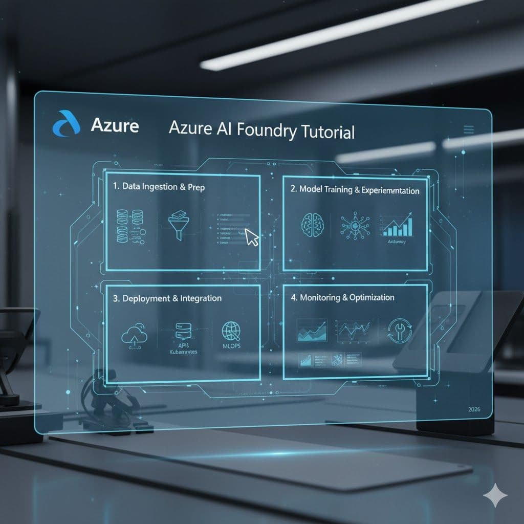
What Is Azure AI Foundry? Complete Getting Started Tutorial
Azure AI Foundry is Microsoft's unified enterprise platform for building AI applications. Learn setup, deployment, RAG implementation, and security with this step-by-step tutorial.
How Do Agentic AI Workflows Transform Enterprise Automation?
Agentic AI workflows are autonomous systems where AI agents independently plan, reason, and execute business processes. Organizations report 40-60% faster operations and 250-400% ROI.
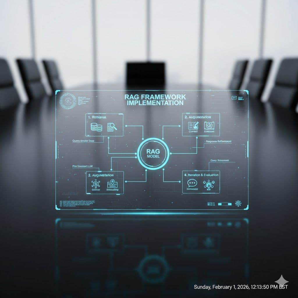
RAG Framework Development: Complete Implementation Guide
RAG framework development combines LLMs with knowledge retrieval to deliver accurate, fact-based AI responses grounded in your data, reducing hallucinations by up to 85%.